Introduction to Data Warehousing - The Data Distillery

What is a Data Warehouse?

A data warehouse is a system where data from various sources are collected, integrated, cleansed, and stored.

The data warehouse has many benefits for an organization. For example, it provides access to information in a timely manner and it can be used to answer questions that may arise during the decision-making process for the company. The data warehouse can also be used to make better decisions in the future by analysing patterns found in the past.

Overview

What is a Data Warehouse?
Data Warehouse Architecture
OLAP Cubes
Storage Technology
ETL Demonstration

Business Database Case Study

Let’s say we have a company with requirements that supports the following activities:

Customers – should be able to find products and create new orders
Inventory – staff should be able to stock, retrieve and re-order goods
Delivery – staff should be able to pickup and deliver goods
HR – should be able to assess performance of staff
Marketing – should be able to attract new customers
Management – should be able to monitor sales growth

Question: Can we build a database to support all of these activities?

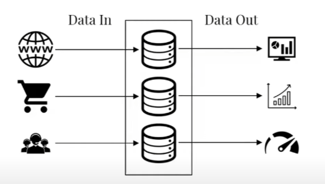
Though our database can store all this information, the activities performed on the database may not necessarily be of the same nature.

The first 3 points are typically of an operational nature, whereas the last 3 points are of an analytical nature.

Why is this differentiation important?

In the above use case, I gave a distinct example between Operational and Analytical use cases. This is a very important point as operational databases are typically handling high I/O load and are far more transactional than an analytical database.

The typical fit, form, function for transactional databases are databases like MySQL, PostgresSQL, or any common relational database like Microsoft SQL or Oracle as they are very good at read and write speed in real time.

If we try and use these databases for analytical purposes, especially for tremendously large datasets we can run into performance issues when performing calculations on many tables with complex joins over a lengthy time period for the analysis.

Hence the latter example is where Data warehousing truly shines, commonly used to leverage our data and tell its story through visualisations, reports, trends and insights enabling us to support analytical processes.

Two common Data warehouse Processing modes are OLTP (Online Transactional Processing) and OLAP (Online Analytical Processing), enabling fast and intuitive access to centralised data for the purposes of analysis and reporting.

Essentially, a data warehouse is a copy of transaction data specifically structured for querying, reporting and analysis.

Data Architecture & ETL Models

To understand the data pipeline we should first consider what it means to solve problems.

We have some problem we wish to solve (input), and some solution to that problem (output), and in between is this black box where we perform some magic that allows us to solve problems.

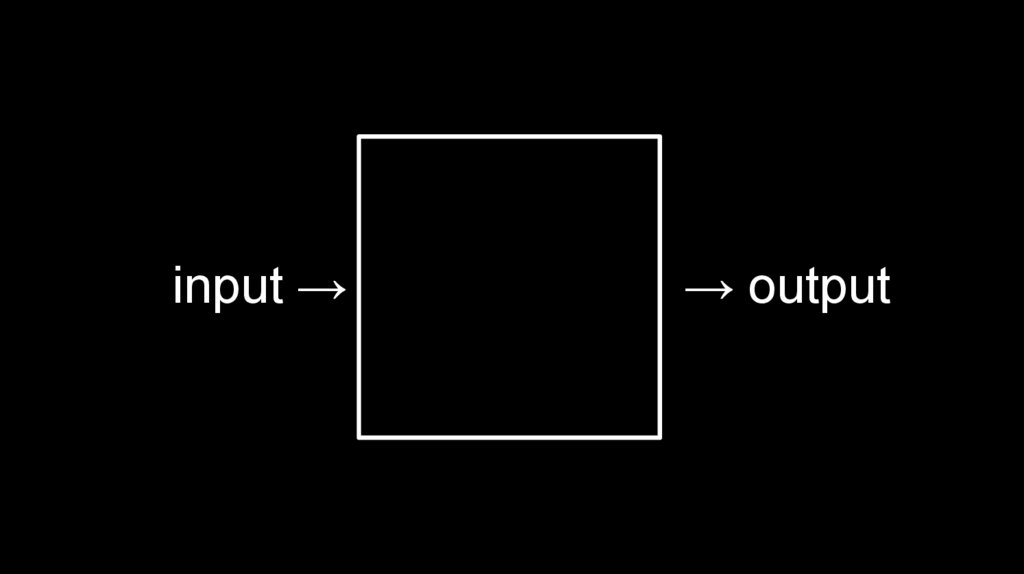
In basic computer science terms, that “magic” is typically an algorithm, or code or process that we perform to get our desired solution.

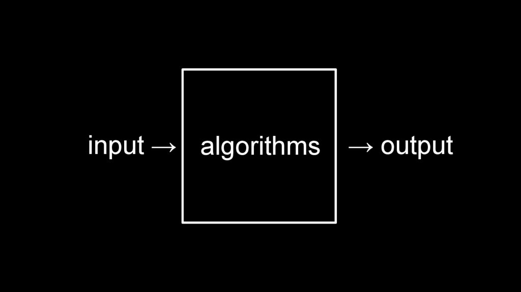
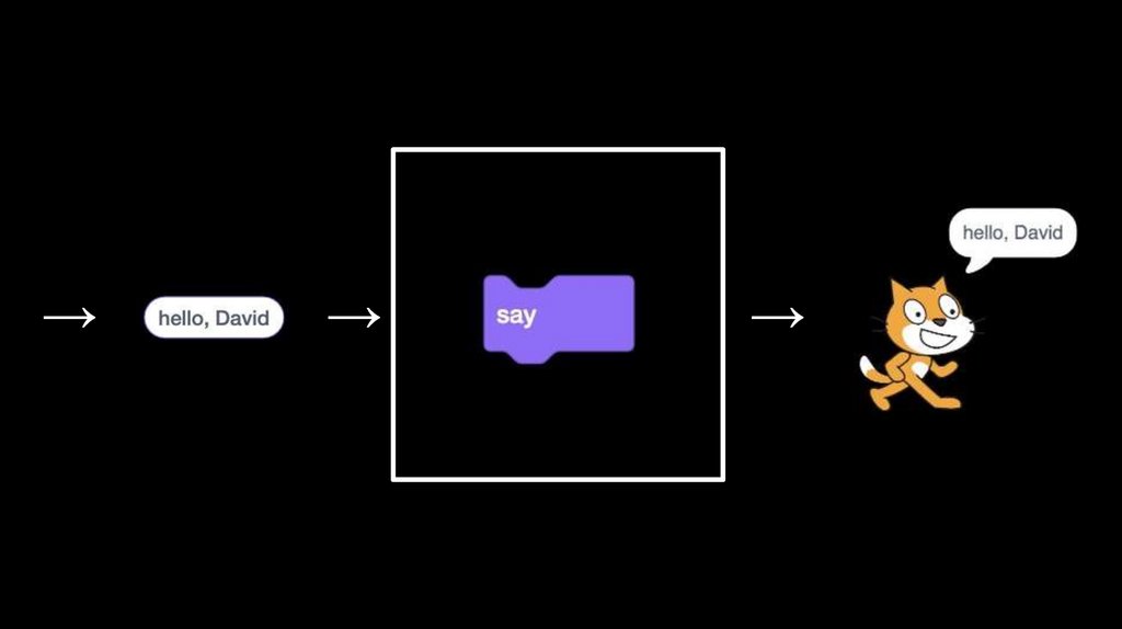
When talking about it in the context of Data Analysis and Data Warehousing, we often will have some form of a problem we’d like to solve for example we want to understand how many people order our products after launching a marketing campaign for ROI.

Input: eg. Customer Orders placed, collected over a certain period of time which gets stored in a database on a server

Process: Extract, Transform and Load (ETL) that transactional data and reformat it into a dimensional model and perform analysis.

Output: A visual data story that provides insights as to whether our marketing campaigns are effective or not, allowing us to make better data driven decisions.

The ETL part of the data pipeline typically is done by extracting data from a data source (database, excel spreadsheets, scribbles on a napkin, etc.), followed by transforming that data into what we need by applying some form of logic using programming languages like Python, R, etc. or tools like Alteryx, Informatica, etc. and finally load that transformed data into a Dimensional Model or Data Warehouse.

A Dimensional Model is something that makes it easier for business users to work with data. A typical database will have its information spread across multiple tables with many different fields of information – this is difficult for your average Joe to decipher, and from a technical point of view it’s not great for performance analysing large datasets spread across multiple tables with many joins and complex queries needed.

The output or solution to our problem is typically displayed in the form of a report or visualisation using tools like PowerBI, Google Data Studio, Tableau, etc. which seamlessly connect to the data warehouse and its special architecture to easily display our required insights.

Dimensional Modelling

So why do we need Dimensional Modelling, and what is it?

Dimensional Modelling makes data intuitive and easy to understand
Fast for analytical query performance

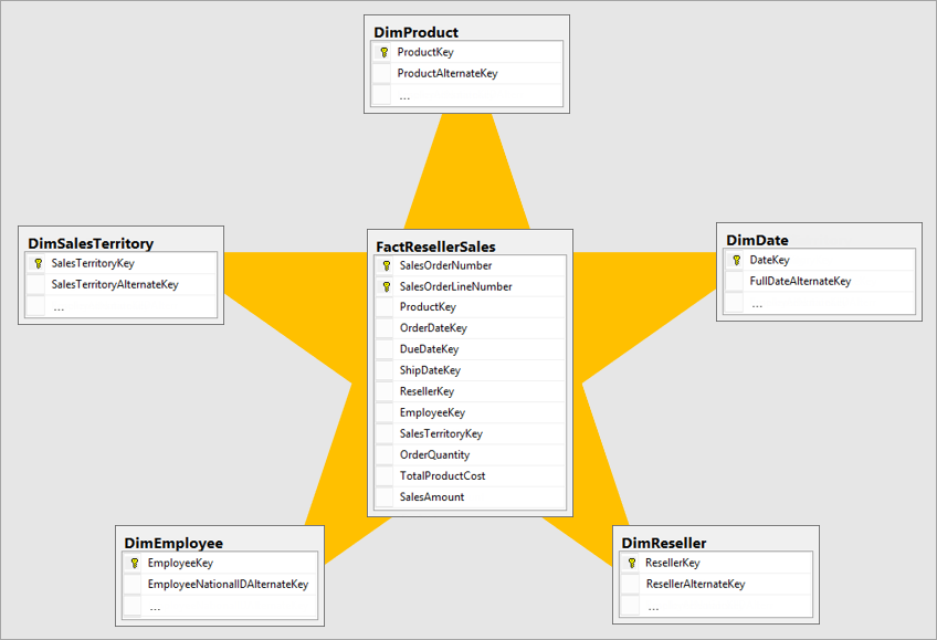
Essentially, Dimensional Modelling (DM) is a data structure technique optimised for data storage in a Data warehouse and consists of “fact” and “dimension” tables.

Fact tables are designed per business process and store purely numerical facts (or transaction data) that are commonly aggregated for reporting purposes and link to dimension table through foreign key fields.
- Fact tables columns record events recorded in quantifiable metrics, like quantity of an item, duration of a call, book rating, etc.
Dimension tables store the descriptive attributes of entities across the business enterprise and function as common lookup tables e.g. product categories, team names, customer names, addresses etc.
- Records the context of the business events, e.g. who, what, where, why
- Dimension tables columns contain attributes like the store at which an item is purchased, or customer who made the order etc.

For facts, If you’re unsure if a column is fact or dimension then simple rule is that fact is usually: Numeric & Additive

Examples facts:

A comment on an article represents an event, however we cannot easily make a statistic out of its content (Not a good fact)
Invoice number is numeric, but performing math on it does not make sense (Not a good fact)
Total amount of an invoice could be summed up towards total sales (A good fact)

Example Dimensions:

Date & time are always a dimension
Geographical location and their attributes
Human Roles like customer and staff
Products sold always good candidates for dimensions

Joins with Dimensional Data Modelling are only good for OLAP, not OLTP

Brief overview of Normal Form Data Models

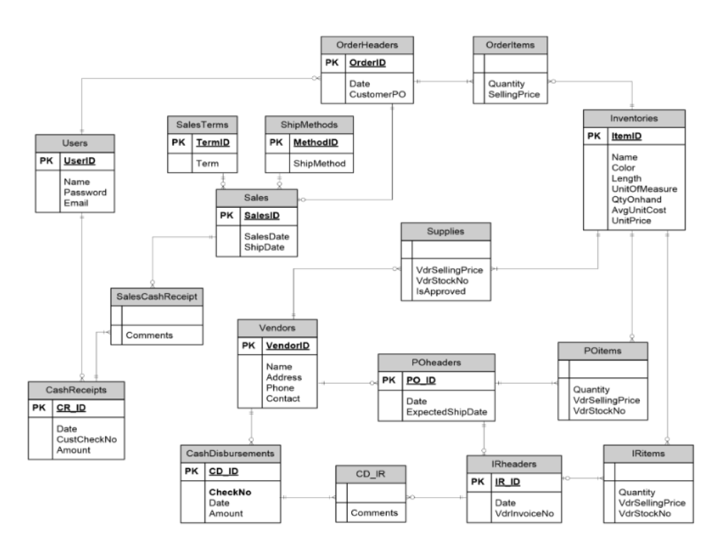
A typical transactional database (relational database) is used to store discrete, business transactional data e.g. sales, inventory, PO’s etc. Each database is specific to a particular business or business functional area (Sales, Marketing, HR, Engineering). In database terminology the typical data model involved with these databases is called the 3rd Normal Form (3NF).

Normal form databases simply refer to the level of safety applied to a database architecture structured in a way to avoid bad or redundant data. A great explanation can be found in the following video: https://www.youtube.com/watch?v=GFQaEYEc8_8

Relational Data Models are great for individual CRUD operations, however very expensive on performance in the context of performing Data Analysis, eg. performing any mathematical or statistical function millions of rows of data spread across many tables.

Demo

For this demonstration I’m running Windows Server 2019 (Eval) in a virtual environment with Postgres SQL

You can download and install here:

https://www.microsoft.com/en-us/evalcenter/evaluate-windows-server-2019
https://www.virtualbox.org/
https://www.pgadmin.org/download/pgadmin-4-windows/
https://www.postgresql.org/download/windows/

Postgres provides a free dataset which you can download here:

https://www.postgresqltutorial.com/postgresql-getting-started/postgresql-sample-database/

This is essentially the “Hello World” of data sets for Postgres, similar to Adventure Works on Microsoft SQL.

You can load the sample dataset into postgres by following this tutorial: https://www.postgresqltutorial.com/postgresql-getting-started/load-postgresql-sample-database/

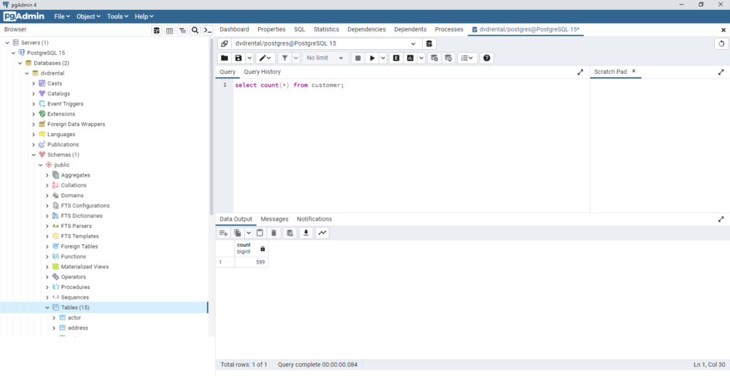
Run a couple queries on the data:

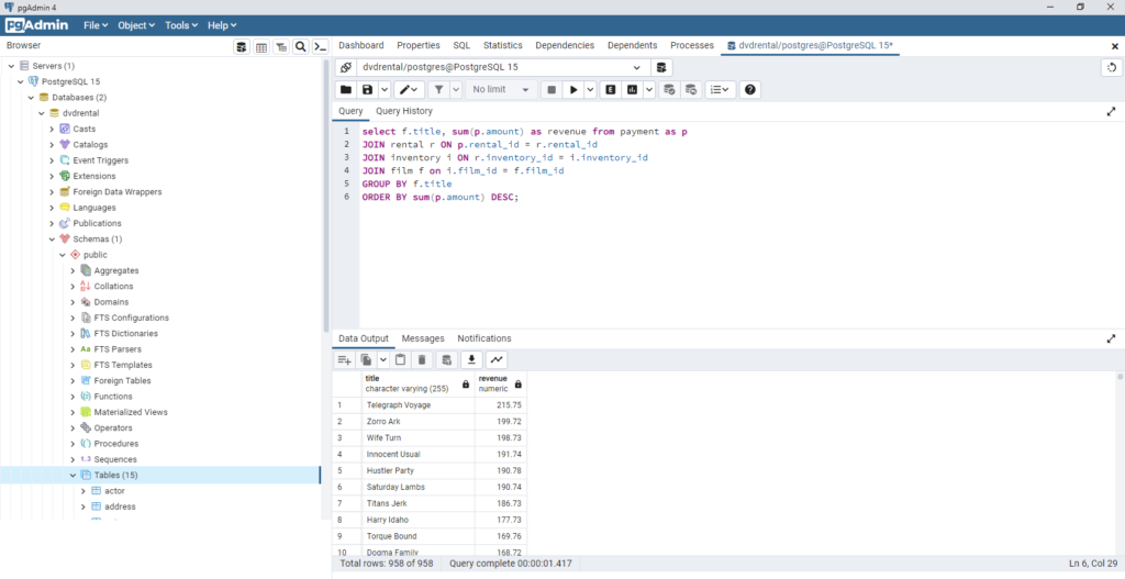
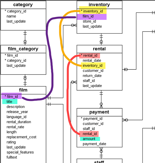
Performing some data analysis – Question: How many sales did we make per film?

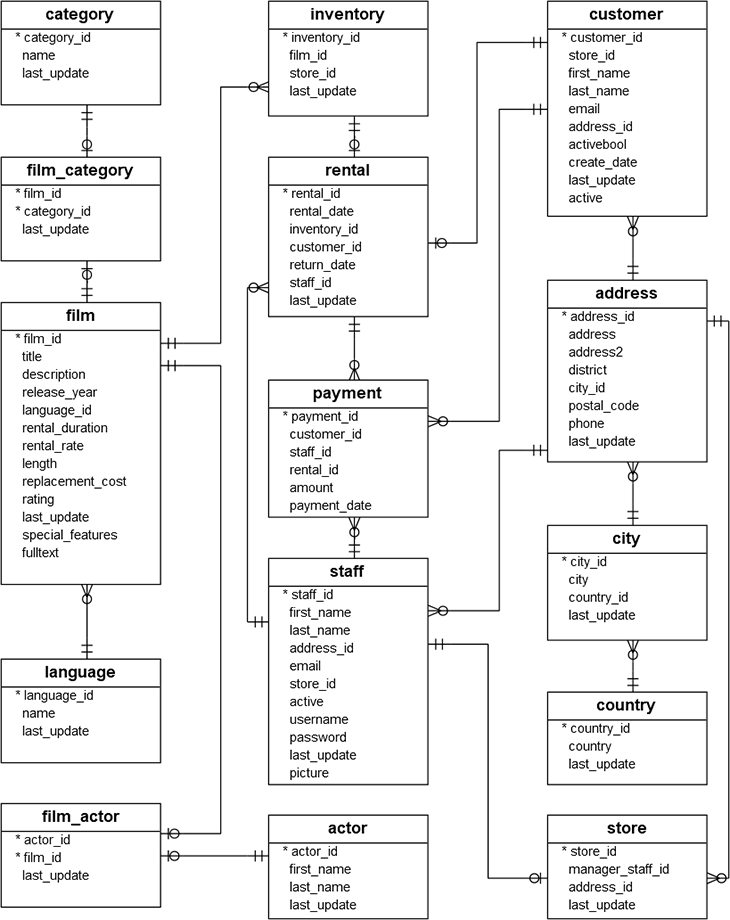
As there isn’t a single table with this data, we need to perform several joins to get this information. We can graphically see this in the above Entity Relationship Diagram (ERD) by going through the Payment -> Rental -> Inventory -> Film tables to return the intended result.

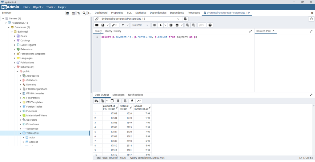
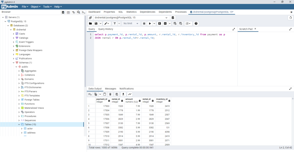
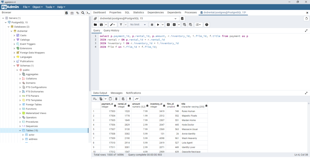
SQL Query

				
					select f.title, sum(p.amount) as revenue from payment as p
JOIN rental r ON p.rental_id = r.rental_id
JOIN inventory i ON r.inventory_id = i.inventory_id
JOIN film f on i.film_id = f.film_id
GROUP BY f.title
ORDER BY sum(p.amount) DESC;

Building out a Star Schema for Data Warehousing & Analytics

Taking the fundamentals learned above, we’ll convert the 3NF Relational Database Model into a Star Schema for Data Warehousing. Firstly I break out the tables into the fact and dimension tables and draw them using a tool like Visio or app.diagrams.net

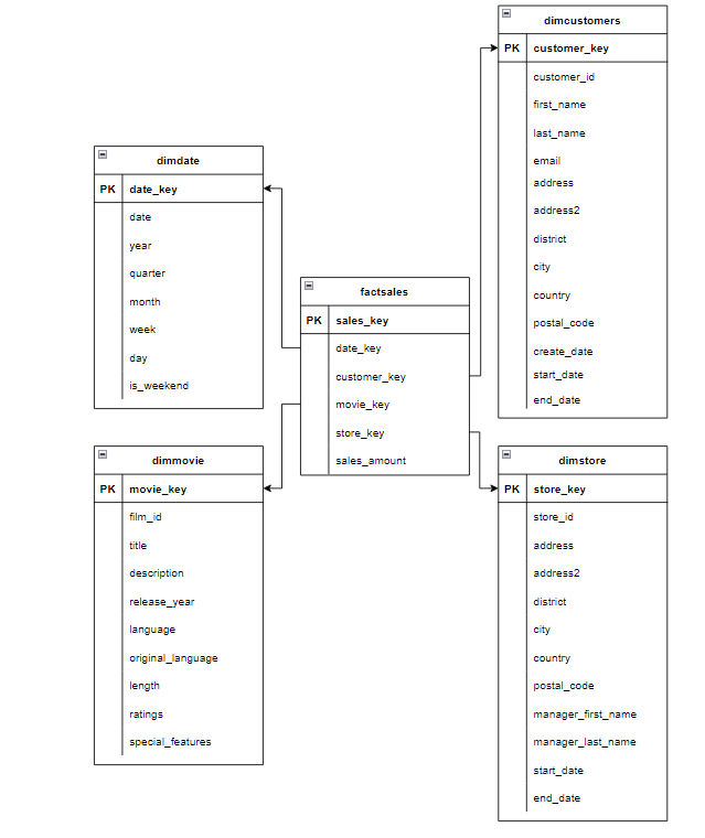
To create this in our SQL Database, we just need to run a simple query to create the tables.

Note: better practice is to create this in a new database.

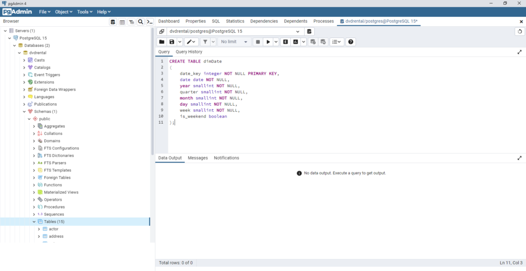
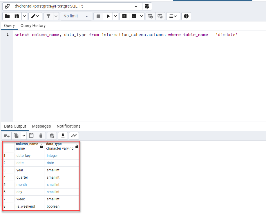
We can take a look at the table schema to validate data types with the following query:

				
					CREATE TABLE dimCustomer
(
  customer_key		SERIAL PRIMARY KEY,
  customer_id		smallint NOT NULL,
  first_name 		varchar(45) NOT NULL,
  last_name 		varchar(45) NOT NULL,
  email 	    	varchar(50),
  address 	    	varchar(50) NOT NULL,
  address2 	    	varchar(50),
  district 	    	varchar(20) NOT NULL,
  city 	    		varchar(50) NOT NULL,
  country 	    	varchar(50) NOT NULL,
  postal_code 		varchar(10),
  phone 	    	varchar(20)NOT NULL,
  active 	    	smallint NOT NULL,
  create_date       timestamp NOT NULL
  start_date 		date NOT NULL,
  end_date 		    date NOT NULL
);

CREATE TABLE dimMovie
(
  movie_key		    SERIAL PRIMARY KEY,
  film_id		    smallint NOT NULL,
  title			    varchar(255) NOT NULL,
  description		text,
  release_year		year,
  language		    varchar(20) NOT NULL,
  original_language	varchar(20),
  rental_duration	smallint NOT NULL,
  length		    smallint NOT NULL,
  rating		    varchar(5) NOT NULL,
  special_features	varchar(60) NOT NULL
);

Create TABLE dimStore
(
  store_key	        	SERIAL PRIMARY KEY,
  store_id	        	smallint NOT NULL,
  address	        	varchar(50) NOT NULL,
  address2	        	varchar(50),
  district	        	varchar(20) NOT NULL,
  city		        	varchar(50) NOT NULL,
  country		        varchar(50) NOT NULL,
  postal_code	        varchar(10),
  manager_first_name    varchar(45) NOT NULL,
  manager_last_name     varchar(45) NOT NULL,
  start_date		    date NOT NULL,
  end_date		        date NOT NULL
);

Now we have our Star Schema tables setup, we can insert data from our relational 3NF tables.

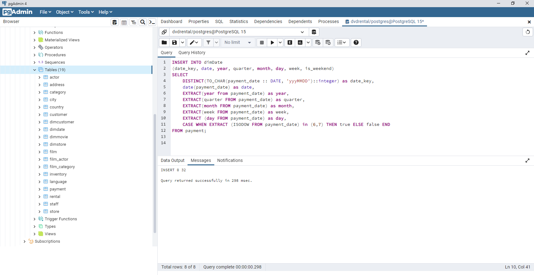
Check the data was inserted correctly:

				
					select * from dimDate;

Insert data into dimCustomer table:

				
					INSERT INTO dimCustomer(customer_key, customer_id, first_name, last_name, email, address, address2,
						district, city, country, postal_code, phone, active, create_date, start_date, end_date)
SELECT	c.customer_id as customer_key,
		c.customer_id,
		c.first_name,
		c.last_name,
		c.email,
		a.address,
		a.address2,
		a.district,
		ci.city,
		co.country,
		postal_code,
		a.phone,
		c.active,
		c.create_date,
		now()	AS start_date,
		now()	AS end_date
FROM customer c
JOIN address a ON (c.address_id = a.address_id)
JOIN city ci   ON (a.city_id = ci.city_id)
join country co ON (ci.country_id = co.country_id);

				
					INSERT INTO dimmovie(movie_key, film_id, title, description, release_year, language, rental_duration, 
					 length, rating, special_features)
select f.film_id as movie_key,
	   f.film_id,
	   f.title,
	   f.description,
	   f.release_year,
	   l.name as language,
	   f.rental_duration,
	   f.length,
	   f.rating,
	   f.special_features
from film f
join language l on (f.language_id = l.language_id)

				
					INSERT INTO dimstore(store_key, store_id, address, address2, district, city, country, postal_code,
					 manager_first_name, manager_last_name, start_date, end_date)
select s.store_id as store_key,
	   s.store_id,
	   a.address,
	   a.address2,
	   a.district,
	   ci.city,
	   co.country,
	   postal_code,
	   m.first_name as manager_first_name,
	   m.last_name as manager_last_name,
	   now() AS start_date,
	   now() AS end_date
from store s
join staff m on (m.staff_id = s.manager_staff_id)
join address a ON (s.address_id = a.address_id)
join city ci on (a.city_id = ci.city_id)
join country co on (ci.country_id = co.country_id);

Now all our Dimension tables have been populated, let’s create and populate our Fact table:

				
					CREATE TABLE factSales
	(
		sales_key SERIAL PRIMARY KEY,
		date_key integer REFERENCES dimDate (date_key),
		customer_key integer REFERENCES dimCustomer (customer_key),
		movie_key integer REFERENCES dimMovie (movie_key),
		store_key integer REFERENCES dimStore (store_key),
		sales_amount numeric
	);

This will create our fact table and reference it to all the appropriate keys of our Dimension tables. Let’s insert some data into the fact table:

				
					insert into factSales (date_key, customer_key, movie_key, store_key, sales_amount)
select
	TO_CHAR(payment_date :: DATE, 'yyyMMDD')::integer AS date_key,
	p.customer_id as customer_key,
	i.film_id as movie_key,
	i.store_id as store_key,
	p.amount as sales_amount
FROM payment p
JOIN rental r ON (p.rental_id = r.rental_id)
JOIN inventory i ON (r.inventory_id = i.inventory_id);

Our Star schema with Fact and Dimension tables have now been successfully created, populated with data and are now ready for data analysis.

Wrapping up

Below are the queries for the 3NF and STAR database architectures. In this example the STAR schema is much cleaner with less joins, and performs 20-25% faster on query time.

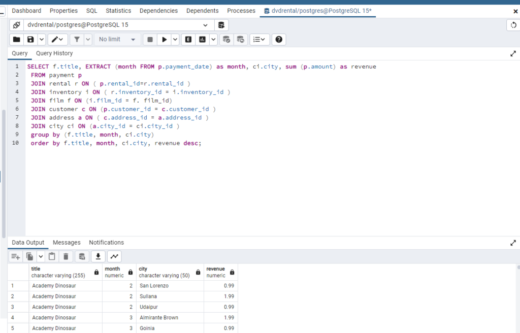
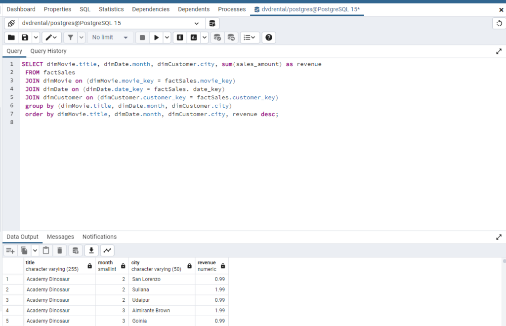
As this is a relatively small dataset the queries both run quite quickly, however as our datasets grows and scales up with more users, customers, products, etc. the longer it can take to perform complex queries on our dataset, especially for data analytics, data science and machine learning processes. In Data Structure and algorithms terminology, it has a linear correlation between iterations as a function of time with respect to Time Complexity and Space Complexity

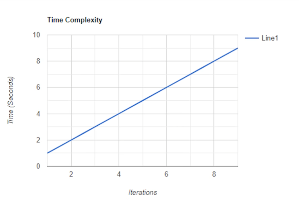
An exaggerated example of this would be if we had a dataset of size 6 that takes 1 second to query each iteration, it would take 6 seconds for the query to complete. If this scaled up to 6000, it would take 6000 seconds.

Now when we add an extra layer of iterations through relationships and joins causing potentially exponential time increases when it comes to data analysis on big data.

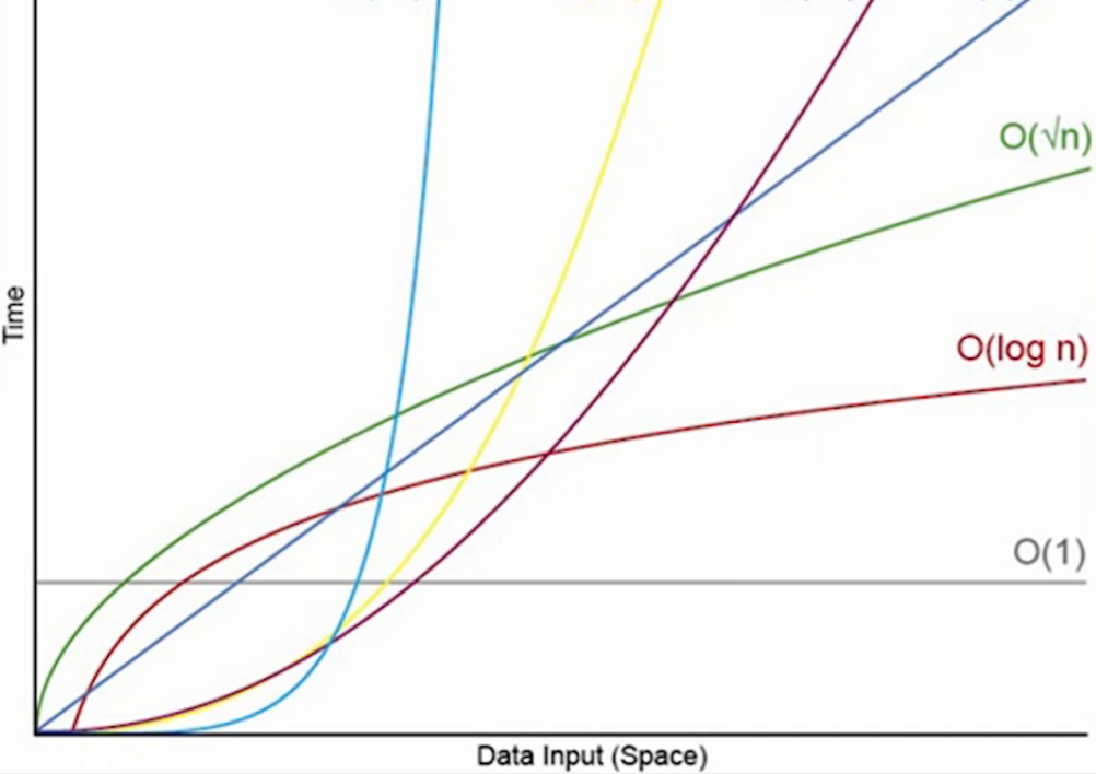
So it’s our job as a Data Analyst to look at a solution with time and space complexity in mind as the data set grows, hence why it’s important to understand the fundamental concepts of data warehousing to develop optimal solutions for the problem that we’re given.